Ed25519 Cryptography - Part 1

This post is an exercise in digesting A Tutorial on Elliptic Curve Cryptography by Martin Kleppmann.

In the first part, we will unpack the Finite Field arithmetic. We will implement basic operations such as addition, subtraction, multiplication, and modular inverse. In the next part, we will implement elliptic curve operations for the signature scheme. The original paper used C. I have instead used Rust. However, the following code snippets only use rudimentary language features in order to focus on lower level operations. Needless to say, this code is only for illustration purposes and should not be used in production.

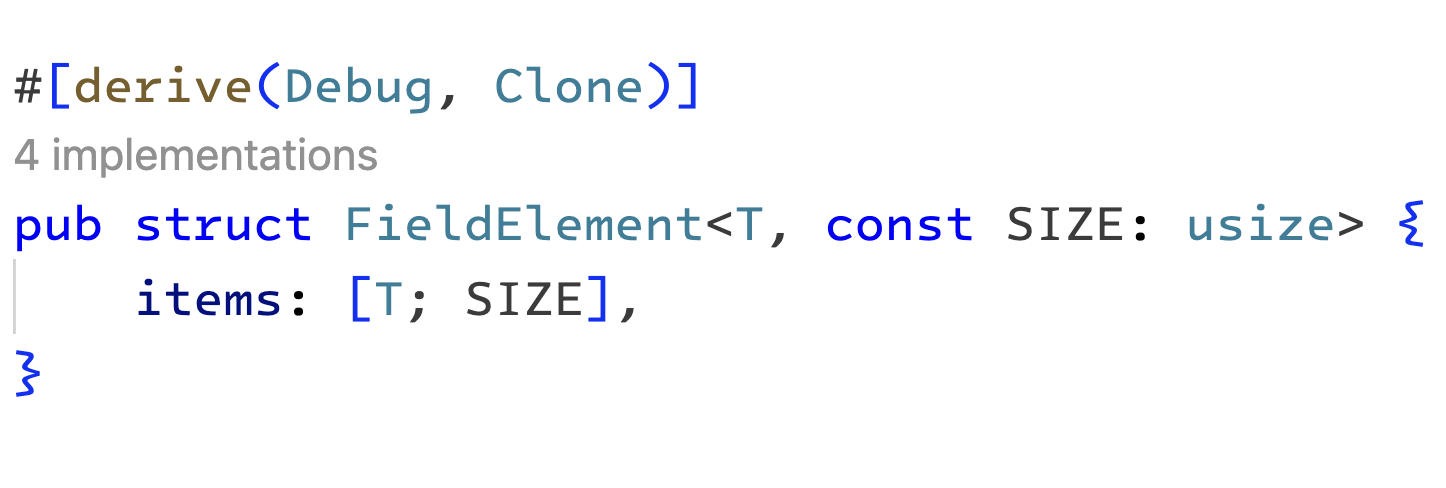
Before we begin, we should take note of two different data types used here. A Field element is represented as a byte array of 32 bytes in the packed form. In the unpacked form, it will be represented as an array containing 16 elements, each 16-bit wide. The size of a Field element is 256 bits in both representations.

Note: we will use an i64 type for each element in the unpacked array. The remaining bits will be left empty initially. This extra space ensures that we are not risking overflows when performing additions and multiplications

The field struct

We will perform arithmetic operations such as addition, multiplication, and inverse in the unpacked form and finally output our result in the packed form to save space.

The most important thing to remember is that any algorithm we implement must be constant time (i.e., O(1)) relative to the input size. Constant time algorithms are more performant and less vulnerable to attacks. If the execution time of cryptographic operations depends on its inputs, then it can be analyzed and reverse-engineered. A cipher system using such algorithms can be broken, leading to dire consequences.^[1]

Addition and Subtraction

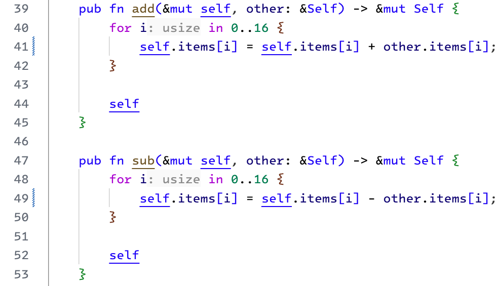
Addition and Subtraction implementations are straightforward. We iterate over our Field array and perform an addition or subtraction operation at every index.

At this point, we will ignore the possibility of a "carry" or a negative result (where the most significant bit is 1). Remember, we are using an i64 array to represent one Field element. We can count on the unused bits to handle these scenarios. Later, when we convert the result to the packed format, we will deal with the carry and negative results.

add and sub methods for finite field elements

Carry

Before we get to multiplication, we should consider handling the carry bits. In the unpacked format, each array element is an i64 integer. Out of which, we have only used 16 bits.

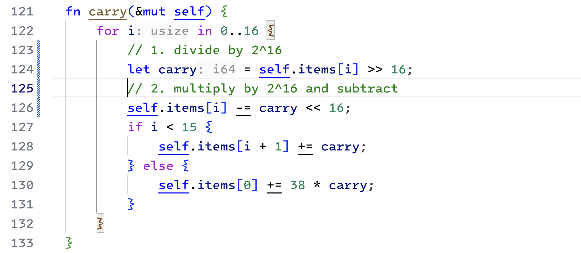
Here is how we will handle carryovers. We iterate over the items of the Field element array and divide each integer by $2^{16}$. There is a carry if the division doesn't make all the bits 0. We move the carry over to the subsequent element.

carry method used in addition and multiplications

If we find carry bits in the last (15th) element, we add that back to the first element, but only after multiplying the carry by 38. The number 38 seems arbitrary. We must look at the multiplication algorithm to understand its origin. So, stay tuned.

Calling this function once can cause the element at the first index to exceed $2^{16}$ or even become negative (due to a wrap-around). A second call can fix this. However, if items between the 1st and 15th index are close to $2^{16}$, the carry bits from the 0th index can cause a cascade of carries. It will result in a further carry from the last element to the first, causing it to exceed $2^{16}$ again.

We must call the carry function three times to ensure no carry bits are left in the Field element. Such a carry cascade is no longer possible on a third call since the middle values are now zero.

Multiplication

Now we are ready to look at multiplication. In the Ed25519 curve, the parameter $p$ is set to $2^{255}-19$. It is the prime modulo of the Finite Field underlying elliptic curve^[2]. In practice, all the arithmetic operations on the Field are done modulo $p$.

Since $p+19$ is $2^{255}$, therefore $2p+38$ is $2^{256}$. There are two points to note here.

First, the size of our data structure is $2^{256}$. It means that reducing any value by modulo $2^{256}$ is easy. Bigger values will automatically overflow.

Second, in the multiplication function, we can get away by reducing the result by modulo $2p$ as long as we later reduce it by $p$. We will do so while packing our result into a byte array before returning the final result.

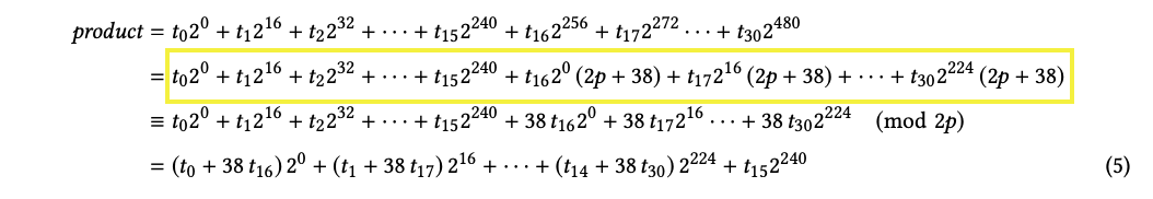
We start the multiplication by taking the product of inputs (in the unpacked form) element by element. We store the individual results in the product array so we can add that up to get the final result. This representation is equivalent to a reduction modulo $2^{256}$ or $2p+38$.

product calculation expressed algebraically

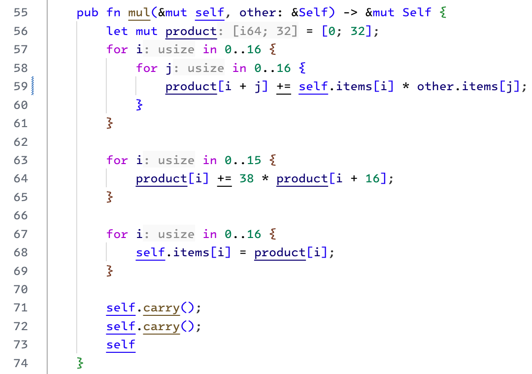
After doing some modulo arithmetic, as shown in the figure above, we can arrive at the equation $5$. Note how the higher powers of $2$ are reduced because of the modulo $2^{256}$ in step 2. Finally, the reduced powers are grouped in step 3. The same thing is implemented below on line 63. We can now ignore the elements between product[16] and product[30] in our initial array.

Finally, we call the carry function twice. It is good enough to account for carry bits and ensure each array element doesn't exceed the 16-bit size.

The multiplication method for finite fields

Fermat's Little Theorem

In Finite Field arithmetic, in place of division we have the modular inverse. The modular inverse of $a$ is $b$ if by multiplying $a$ with $b$ in the given modulo, we get $1$ (multiplicative identity of the field).

Fermat's little theorem says the following. Here, $p$ is a prime and $a$ is any integer.

$$a^{p-1}\equiv 1\mathrm{mod}p$$

For our purpose, $p=2^{255}-19$. We can use the formula to find the inverse of a given field element.

Modular inverse

Using the theorem, we can see that:

$$a^{-1}\equiv a^{p-2}\mathrm{mod}p$$

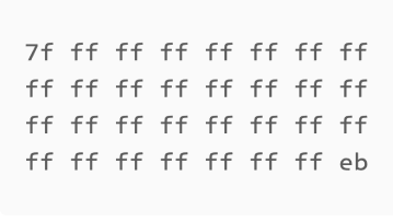
Essentially, we need to calculate $a^{p-2}modp$ where $a$ is the given field element. And $p-2$ is $2^{255-19-2}$. In hex, $2^{255-21}$ is represented as:

bytes in $p$ i.e. $2^{255}-21$ shown in hexadecimal

The hex notation makes it easy to see that besides the first and the last byte, all other bytes are ff (i.e., all 8 bits of a byte are 1). If we look closer at the first and the last byte, we notice that 0x7f = 01111111 and 0xeb = 11101011. It means that all the bits of $p-2$ are 1 except the 2nd, 4th, and the most significant bit.

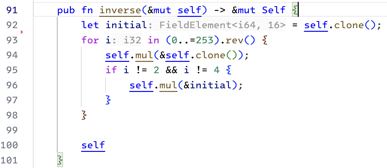
Here is the inverse algorithm. We iterate in a loop $254$ times and maintain an accumulator in the result variable. We will initialize this accumulator with the input (line 91).

The inverse method for finite fields

In every iteration, we will square the accumulator and reassign the value. Further, if the bit is set for an index (that is, every index except the 2nd and 4th), then we also multiply the accumulator with the input value.

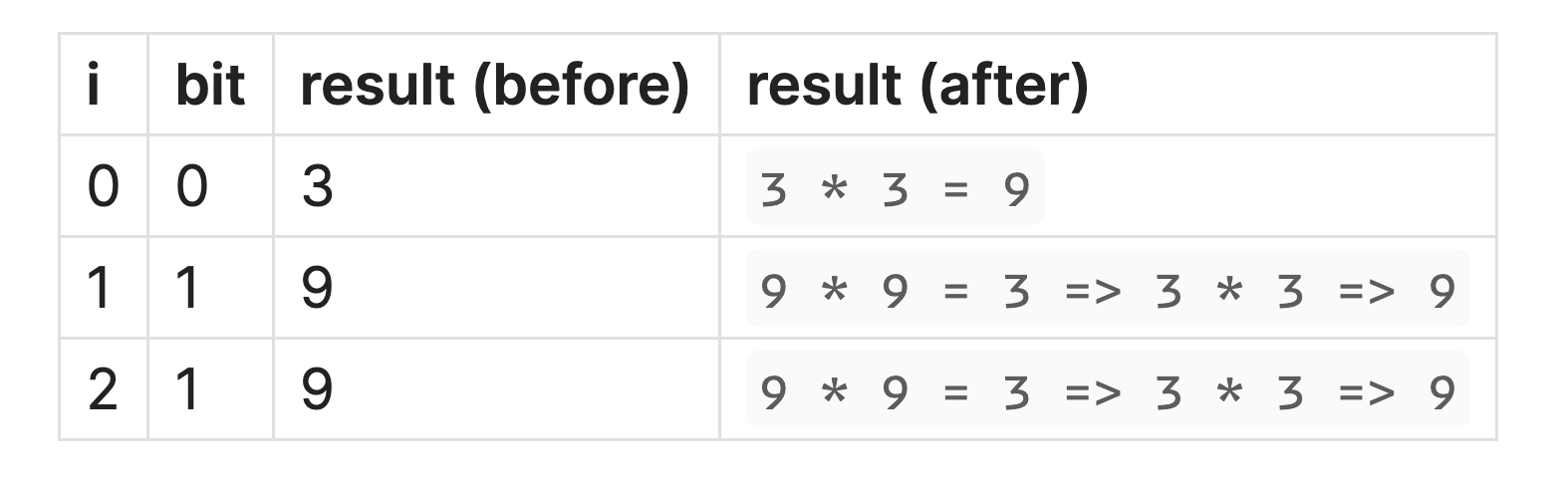
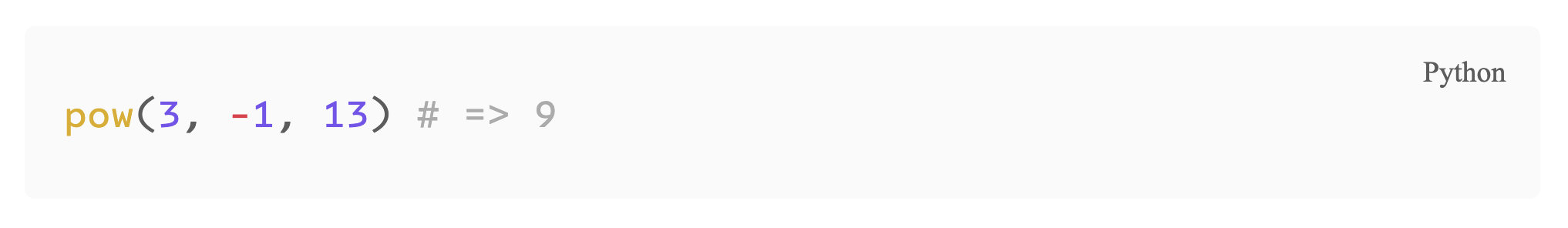
To understand how the algorithm works, we can take a smaller example. Let's say we want to calculate the modular inverse of 3 in the prime field where $p$ is 13. In this case, $a=3$ and $p-2=11$. The binary representation for 11 is 1011. We will initialize the result with 3, skip the most significant bit, and iterate 3 times for the remaining bits: 011.

Mod inverse table

Note: all the multiplications in the above table are in mod 13. We can quickly verify our result in a Python shell

Mod inverse in python

With that, we are done with the arithmetic operations. Next, we will focus on transforming between the two data types we discussed earlier.

Unpacking

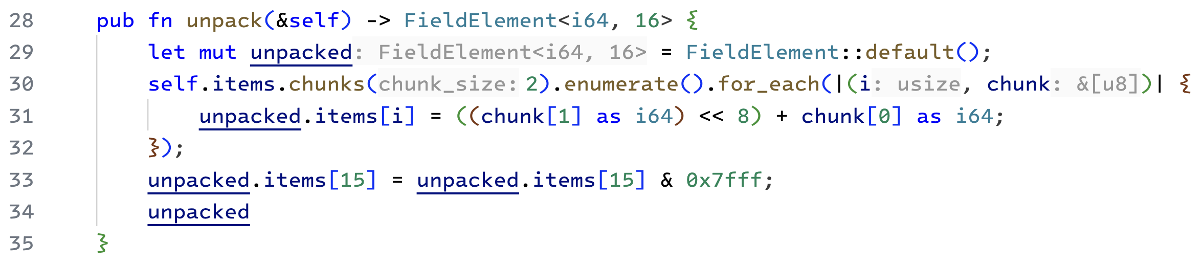
As the name suggests, the unpack function will convert a packed representation (byte array) to an unpacked one. This is straightforward. We start by creating a new Field element. Initialize it with 0 values. Next, we iterate through all 16 elements and update them. We combine two adjacent bytes from the packed byte array into a 16-bit value. To do so, we multiply the 2nd byte by $2^8$ and add them together.

Unpacking the byte array to operate on field elements

Finally, we make sure that the most significant bit is zero. We do this by taking the last element modulo $2^{15}$, since, in our prime field arithmetic, every number is less than $p$ (i.e., $2^{255-19}$).^[3]

Bit Swap

bit swapping

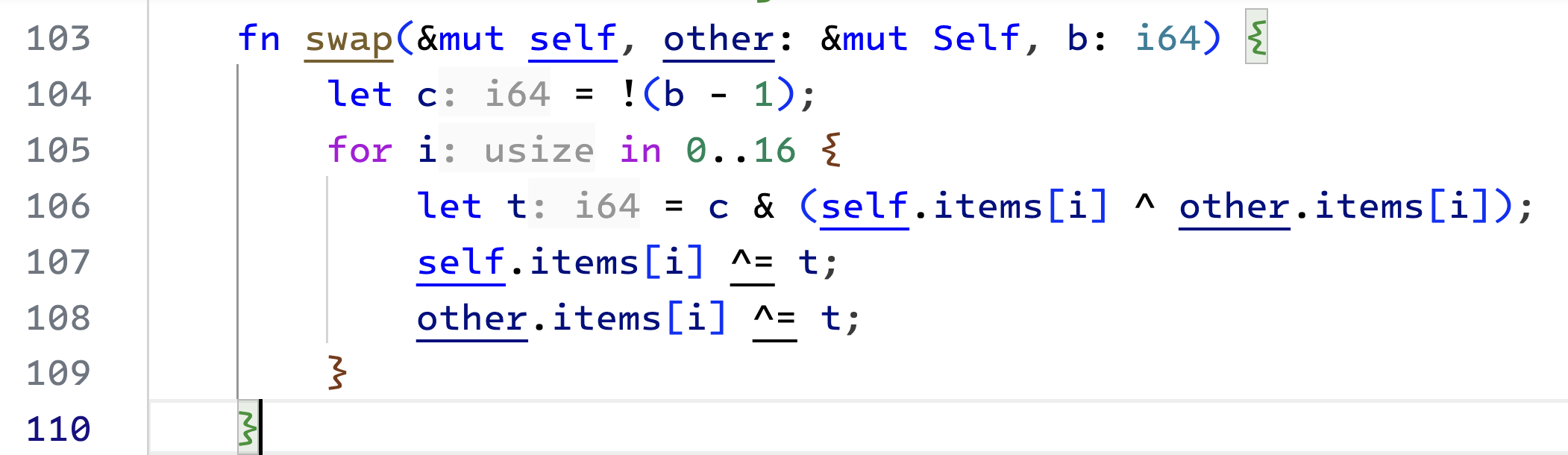
Before we start with the pack function, we need a swap function. It will take two Field elements and swap their bits only if the respective bit of the third argument is 1.

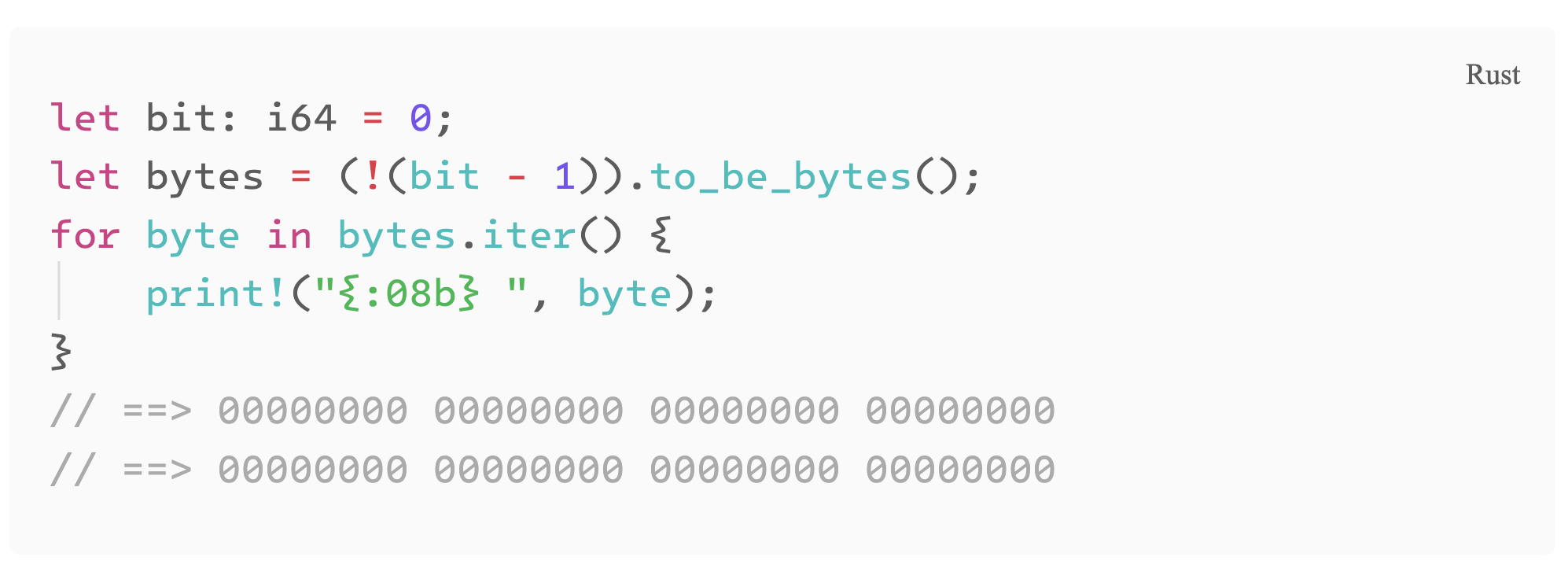
Notice the i64 variable c. Due to the bitwise negation, it will have all its bits set to 1 when the 3rd argument (b) is 1, and all the bits will be 0 when the b is 0. We can print it out to see the memory representation. ^[4]

bit pattern for variable c in bitswap

The bitwise XOR operation will only result in 1 when both of its inputs are different. For each item in the array, we will initialize a temporary variable (line 106). Each bit in this variable will only be set if the corresponding bits of the 3rd argument are set (bitwise and), and the bits of p and q are different (bitwise xor).

Hence t will capture the differences in the bits of p and q. Its bits will be set where the bits of p and q don't match. Finally, if required, the bitwise XOR with t on lines 107 and 108 will flip the bits of p and q.

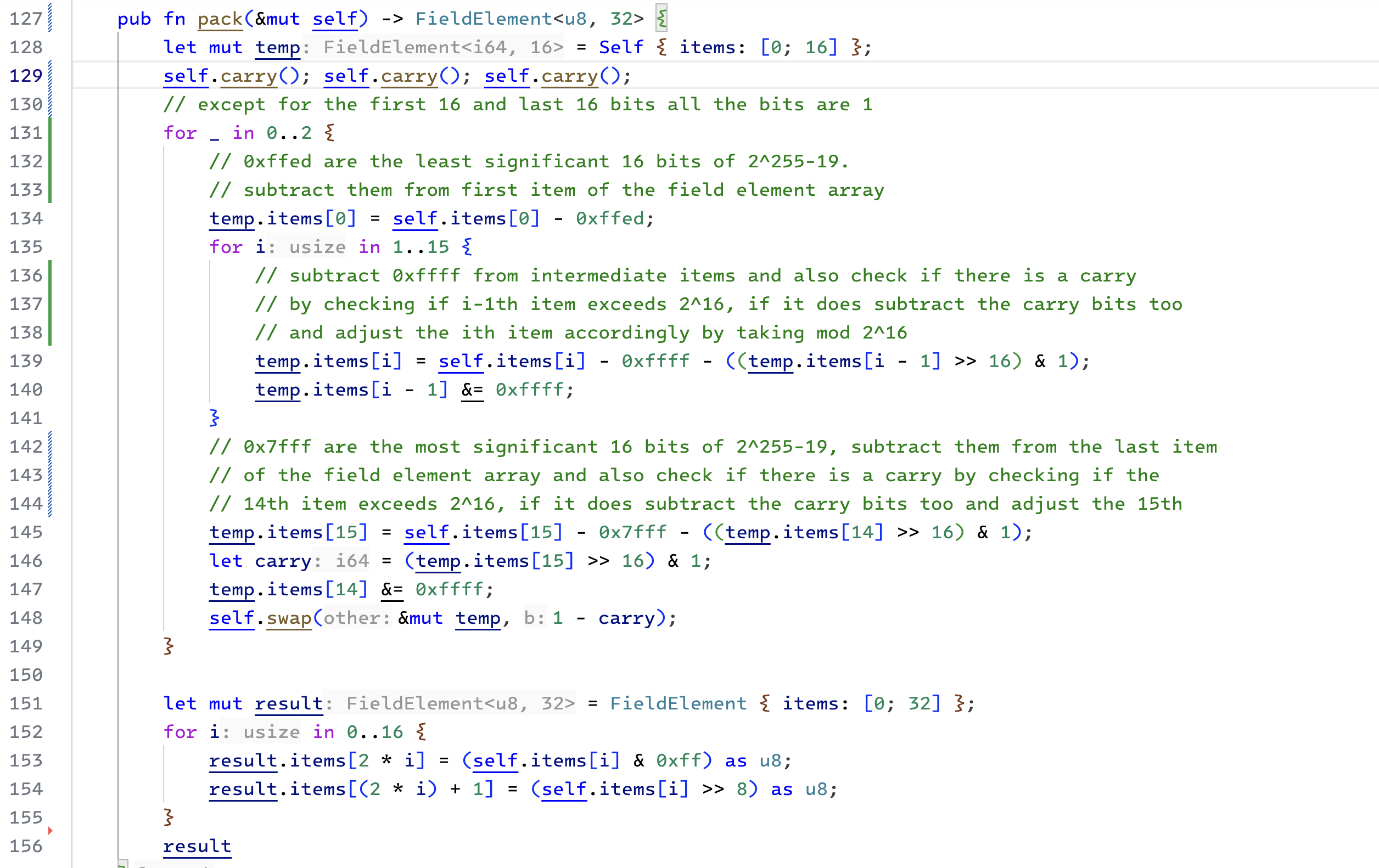
Packing

Packing the Field element array back to the byte array is tricky. We start by first ensuring that none of the elements overflow. We do this by calling the carry function three times, as discussed before.

Recall that earlier, we only reduced our calculations by modulo $2p$. It means that the input value in the pack function can lie between $0$ and $2p$. The next step should be to reduce the input value by modulo $p$. Before we do that, notice that only three possible cases exist. The input value can lie within one of these buckets: $[0,p)$, $[p-2p)$, $[2p-2^{256})$. In the first case, we can pack the input value. In the latter two cases, we must first subtract the input value by $p$ and $2p$, respectively.

We want a constant time algorithm. It cannot depend on the size of the input (i.e. result of our calculation). To find the correct bucket we will subtract by $p$ two times from the result and store our result in an intermediate variable. If the value becomes negative after the first subtraction, we will do the second subtraction anyway but pack the original value (discard the result of the subtract operation). If it becomes negative after the second subtraction, we will use the first subtraction's result (discarding the second subtraction's result). Otherwise, we will pack the output of the second subtraction.

Packing the result into a byte array

We can tell a value is negative if the last item of the field element array is wider than 16 bits. Similar to how we calculate carry bits.

Here, we will use the swap function. If the value is negative (carry = 1), we will not swap the intermediate result of the subtraction in temp with the input. If the value becomes negative in first iteration, it will also be negative after the second iteration. We won't swap again and pack the input. However, if the value is not negative after the subtraction, we will change the original value with the result of the subtraction and proceed with the second subtraction.

Conclusion

With all these functions in place, we have completed the finite field arithmetic required for understanding elliptic curve operations. In subsequent posts, we will use these concepts to implement the Ed25519 signatures.

Notes

1. This book has an excellent account of the impact of using and breaking cipher systems throughout history (see the code book)

2. Check out chapters 4 & 5 from the moon math manual to better understand fields, groups, rings, and elliptic curves.

3. Bitwise & operation is equivalent to taking mod of a power of 2.

4. Check 2s complement binary representation.